Five new built-in contact models have been added to PFC 7.0, for a total of 16 contact models plus the null contact model.
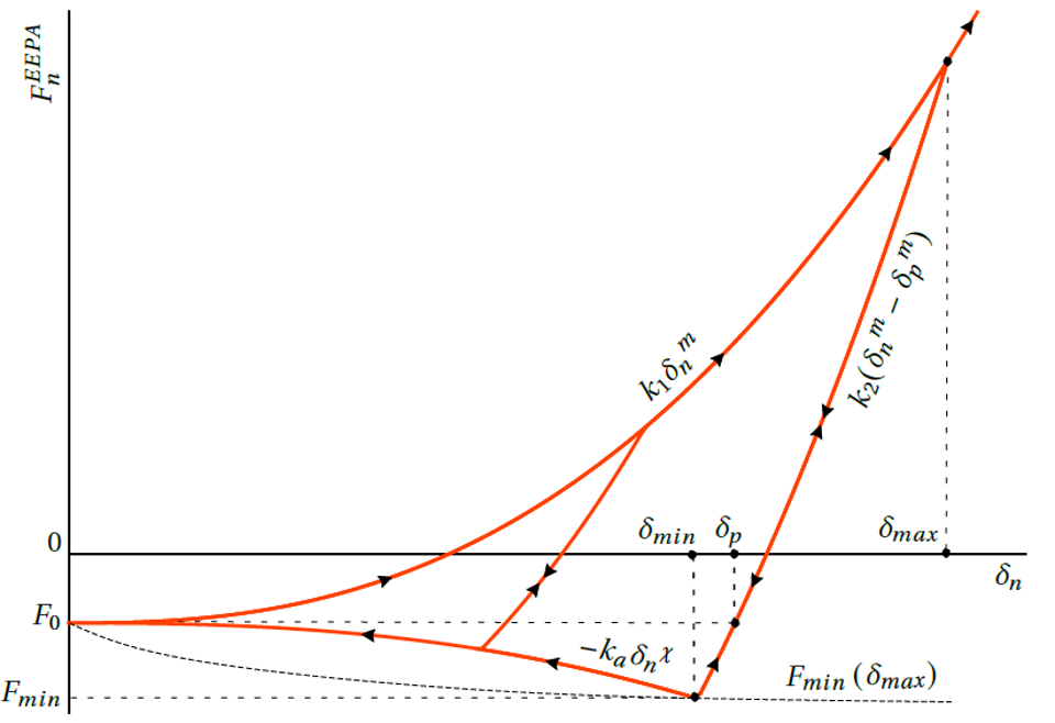
Edinburgh-Elasto-Plastic-Adhesive (EEPA) Contact Model
Material subjected to relatively high loads (consolidation) may experience plastic deformation that results in increased contact area and increased cohesive behavior. History-dependent cohesion (or adhesion) can be modeled in PFC by introducing an attractive force component to the contact model.
The Edinburgh-Elasto-Plastic-Adhesion (EEPA) contact model, developed by Morrisey (2013), is an extension of the linear hysteretic model by Walton and Braun (1986). This model allows tensile forces to develop, and provides a non-linear force-displacement behavior in compression. The model also incorporates viscous damping and rolling resistance mechanisms similar to the Rolling Resistance Linear Model.
Johnson-Kendall-Roberts (JKR) Contact Model
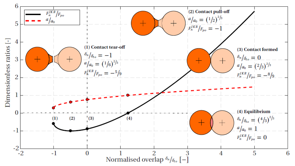
The Johnson-Kendall-Roberts (JKR) contact model is an extension of the well-known Hertz contact model proposed by Johnson (1971). The model accounts for attraction forces due to van der Waals effects. The model is, however, also used to simulate material where the adhesion is caused by capillary or liquid-bridge forces as discussed by Hærvig (2017), Carr (2016), Morrissey (2013), and Xia et al. (2019).
The JKR contact model is an extension of the Hertz-Mindlin model, which allows for tensile forces to develop due to surface adhesion. This model also incorporates viscous damping and rolling resistance mechanisms similar to the Rolling Resistance Linear Model.
Spring Network Contact Model
A spring network bond is a set of elastic springs with constant normal and shear stiffnesses, uniformly distributed over a cross-section lying on the contact plane and centered at the contact point. Relative motion at the contact causes development of a linear force and moment that act on the two contacting pieces. This behavior is the same as the linear parallel bond and the soft-bond model. But unlike those models, a method exists to compute contact stiffnesses that are consistent—when bonded—with an elastic material with a target Young’s modulus and zero Poisson’s ratio. If a non-zero Poisson’s ratio is specified then a fictitious force, derived from linear elasticity, is computed and added to the total force to produce the desired Poisson effect. If the maximum normal stress exceeds the bond tensile strength, the bond may enter a user-defined force-displacement regime before breaking. If the maximum shear stress exceeds the bond shear strength, then it breaks and may enter a user-defined force-displacement regime in the shear direction. If the bond is inactive but the contact is active, frictional strength parameters govern slip with potential dilation and/or healing.
The spring network model can be used to simulate unbonded and bonded systems. The bonded formulation is based on the Rigid Block Spring Network (RBSN) lattice model introduced by Bolander (1998a) and the subsequent work of Asahina (2015) and Asahina (2017). Some key characteristics of this model include:
- the effective removal of particle-scale heterogeneity in elastic response, allowing the user to control heterogeneity;
- the ability to match a target Young’s modulus directly; and
- matching a target Poisson’s ratio.
Rasmussen (2021) and references therein demonstrate the effective use of this methodology in DEM simulations.
No property calibration is needed for macroscopic Young's modulus and Poisson's ratio. Corrections are automatically applied to contact forces based on the current average stress tensor of the contacting blocks and the elastic behavior of the blocks.
In an unbonded state, the spring network model behaves similar to the contact model proposed by Jiang (2015a), providing the ability to transmit both a force and a moment at the contact point, with frictional strength parameters limiting the shear force, bending moment, and twisting moment. Dilation and evolving shear strength as a function of slip can also be specified.
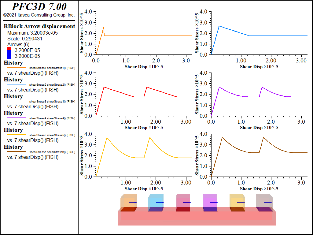
In its bonded formulation, the model behavior is similar to that of a linear parallel bond or soft-bond model, with the possibility for the bond to fail if the bond strength is exceeded either in shear or in tension. Unlike those models, contact properties can be computed based on lattice theory to provide a theoretical match to a target macroscopic Young’s modulus and Poisson’s ratio. Similar to the soft-bond model, the bond may not be removed upon failure in tension. Instead, it may enter into a user-specified softening regime until the bond stress reaches a threshold value, at which time the bond is removed and considered broken. For example, the following figure (left) shows six contact behaviors for different interface/joint conditions: 1) no slip weakening friction, 2) linear slip weakening friction, 3) linear slip weakening with healing, 4) piecewise linear slip weakening with healing, 5) piecewise linear slip weakening with healing and cohesion, 6) piecewise linear slip weakening with healing, cohesion, and residual cohesion.
FISH Contact Model
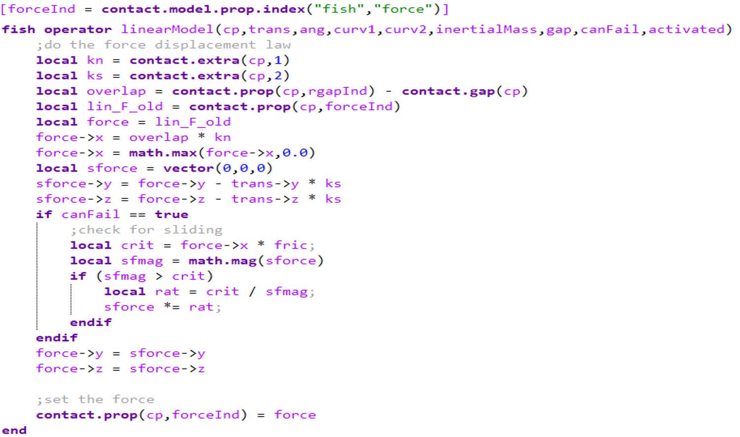
The FISH model does not encapsulate any contact physics. Instead, the user must specify a FISH function that is called during the force-displacement law.
The FISH contact model can be used to facilitate contact model development. The FISH scripting language provides a powerful tool for adding custom physics. This contact model is a blank slate for users to implement their own contact physics via a FISH function. The function must take nine arguments that are filled inside the force-displacement computation. The FISH function must modify the contact model force and/or moment. If effective stiffnesses are provided, then the timestep is determined automatically. C++ contact models and FISH intrinsics are still available.
Contact extra variables or global FISH symbols can be used to manage the contact model properties. It is also strongly suggested that the contact property indices (see contact.model.prop.index and contact.prop.index) be used to set the properties in the FISH model while cycling, as string properties increase modeling times significantly.
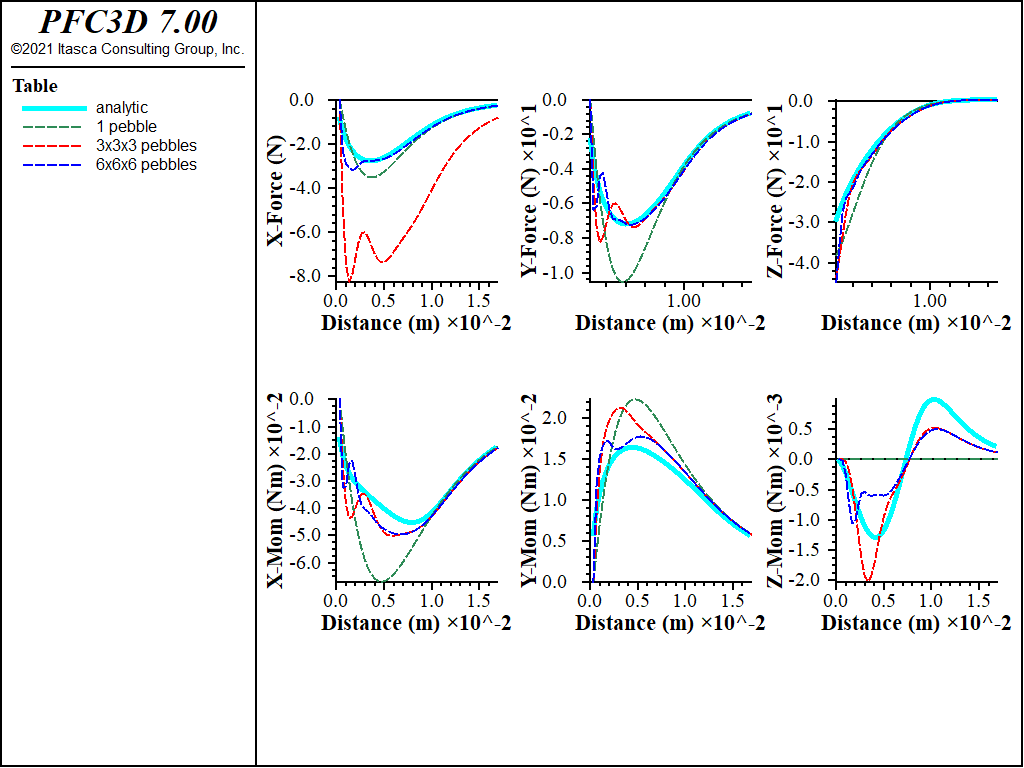
Linear Dipole Contact Model
The linear dipole model is mechanically the same as the Linear Model, comprised of both linear and dashpot components. The linear component provides linear elastic (no-tension) frictional behavior, while the dashpot component provides viscous behavior. Both components act over a vanishingly small area, and thus transmit only a force.
In order to model magnetic interactions, each piece is abstracted as a magnetic dipole based on Thomas and Zewski (2008). Forces and moments due to the dipole interactions are computed and also applied to the pieces. The moments applied to each piece due to the dipole interactions are, in general, not the same. One must also use the proximity concept (see the contact cmat proximity command) so that contacts may be deemed active despite the lack of physical overlap. Inheritance of the dipole_mo surface property is also required along with orientation tracking (see the model orientation-tracking command).
For example, the following figure compares the analytic solution for the attractive forces/moments for square ferromagnets, derived by Akoun (1984), with those produced by the Linear Dipole Model contact model (based on the configuration reported by (Thomas and Zewski, 2008). In this verification problem, a square clump with a 1 cm side is created with various numbers of pebbles. The clumps have uniform magnetic induction of 1 Tesla. The corresponding magnetic moment is set for each pebble accounting for the total number of pebbles. Each pebble must interact with each other pebble of the other clump. The side lengths are 1, 3, and 6 pebbles, resulting in 1, 27, and 216 pebbles per clump and 1, 729, and 46,656 contacts. The model and analytical solutions compare well, improving with increasing resolution (more pebbles used).